BWH-CCDS Data Science Pathway Resource Website
An entry-level resource for Data Science in Radiology
Project maintained by wfwiggins Hosted on GitHub Pages — Theme by mattgraham
Introduction to Python, IPython and Jupyter Notebooks
02 Jun 2019 - Walter Wiggins
Python is a high-level, object-oriented programming language with easy-to-understand syntax. The name was inspired by Monty Python. It is the most commonly used language among data scientists who focus on developing machine learning applications for medical image analysis and natural language processing. For this reason, it is the language we will teach on this site.
If you are new to Python, I suggest you start by reviewing the Beginner’s Guide to Python.
IPython
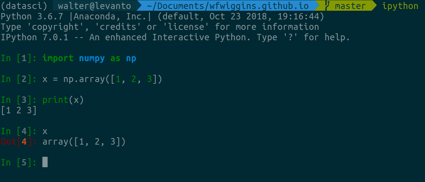
IPython (or Interactive Python) is a “read-eval-print loop” (REPL) programming
environment for the Python language. It is the basis for Jupyter notebooks. It
is a program run via the shell by entering the command ipython, assuming that
you have this package installed. I find IPython to be a very convenient way to
test code and ideas for functions without having to run a script every time.
Some people use Jupyter notebooks for this purpose, but sometimes that gets a
little messy. So…when I’m really experimenting, I tend to open up my Terminal
and run IPython.

Anaconda, conda and virtual environments
The main reason I recommend you install and manage Python via conda is that it
provides the full range of tools for managing Python packages and virtual
environments. What is a virtual environment, you ask? I find it easiest to
think of an env as a contained subset of your programming environment where
the packages you install and any upgrades or downgrades you make are independent
from other environments. In truth, some packages installed in your top-level or
base env are available to you in other envs; however, the version you install
in a given env supercedes the top-level version when it’s go-time. Okay, dude…so
why do I care?
Developing cutting-edge tech means that you will sometimes find yourself using other people’s code that is based on different versions of certain packages that are also required by other packages you use or code you have written. Sometimes a conflict arises, where neither program can work with one of the two versions. Other times, automatic upgrades to packages can break your code due to changes in the available functions in newer versions of that package. Developers are usually nice enough to warn you of their future plans to screw your code by flagging a doomed function with the term “deprecated”. Anyway, these situations are where virtual envs are your friend.
To take a look at what env is currently active, open your shell and enter the following command (again, I’m assuming you have conda installed as per the Setup Guides):
$ conda env list
# Conda environments
#
base        *   /home/walter/miniconda3
You should see something similar to the output above. If you’re thrown an error, go back to the Setup Guide and make sure you follow each step. If you do that and are still getting an error, this is a great time to check-in with your old friend Google and your new pal StackOverflow to see where things have gone awry with your setup.
From here, I assume that your conda distro is working like a charm and you’re
ready to move on. Before we do that, go ahead and save this conda cheatsheet
for future reference when you’ve invariably forgotten the commands I’m showing
you here. OK, now we’re ready to create our first conda env. Enter the commands
below to create a new env called datasci with some basic necessities for
anyone learning data science.
$ conda create -n datasci numpy pandas matplotlib ipython jupyter python=3.6
Note: the above step will install the following Python packages:
- ipython - described above
- numpy - standard numerical computing library
- pandas - data manipulation library (good for managing tabular data)
- matplotlib - basic data plotting library
- jupyter - notebook-style environment
MacOS Users: You will need to run the following commands in your terminal to
get matplotlib working properly.
$ mkdir ~/.matplotlib
$ echo "backend: TkAgg" >> ~/.matplotlib/matplotlibrc
The beauty of conda (and with any good package manager) is that this relatively
simple command will install everything that each of these packages needs - their
dependencies - automatically, ensuring mutual compatibility. There will be a
confirmation at some point asking you to enter “y or n”. Enter y to proceed.
Now that you’ve created your datasci env, it’s time to activate it. MacOS and
Linux require you to enter source activate [env name] to activate a conda env;
likewise, source deactivate to deactivate the current env (without the env name).
I recommend you head over to your .bashrc or .zshrc and create aliases
for these to save you some keystrokes later.
# Aliases
alias activate="source activate"
alias deactivate="source deactivate"
Now enter source activate datasci (or activate datasci, if you set an alias
and remembered to reload your shell) to activate your environment, then you should
see something similar to the following output when you enter the following command.
$ which python
/home/walter/miniconda3/envs/datasci/bin/python
Alright! Now you can launch IPython and code to your heart’s delight…
Jupyter & Jupyter Notebooks
Setting up your datasci env also gave you access to Jupyter notebooks. The
roots of the Jupyter notebook are in IPython, but it behaves a little differently.
For this reason, we’ll first create a new subdirectory within your home directory
called projects and navigate to that directory before launching the program.
After you create your first Jupyter notebook, it will save checkpoints within
a subdirectory called .ipynb_checkpoints/.
$ mkdir projects
$ cd projects
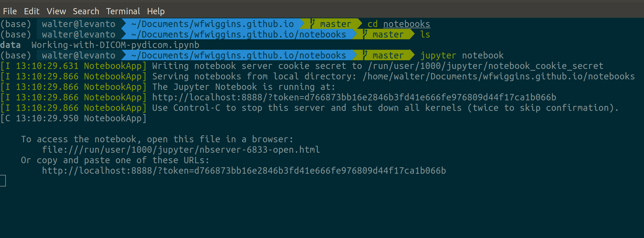
Next, when you run the command jupyter notebook, you convert your shell into a
server that runs the Jupyter program as a web service. On most machines, a web
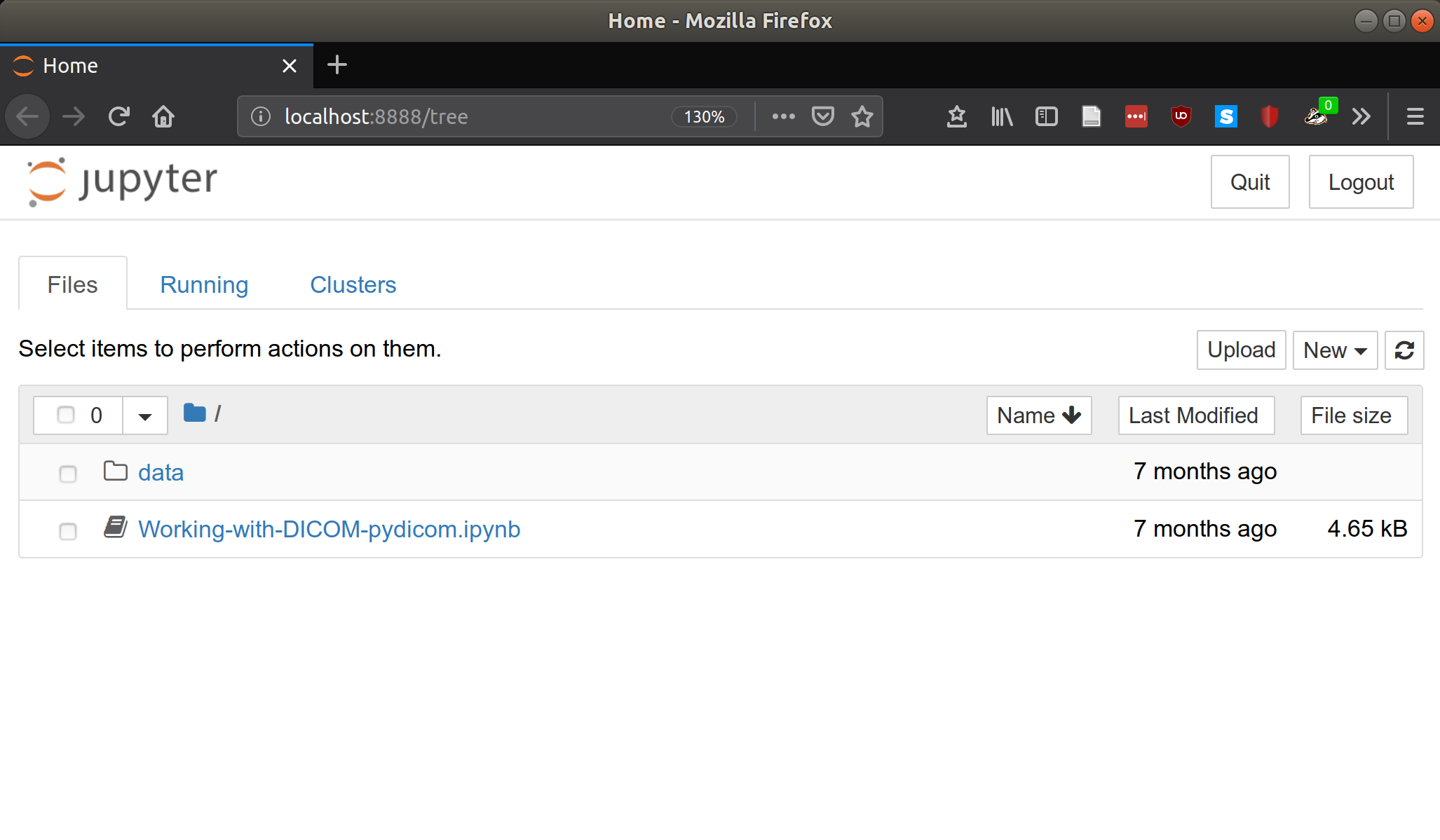
browser window will automatically launch. If this does not happen for you, try
opening a new browser window and typing the following address: localhost:8888.


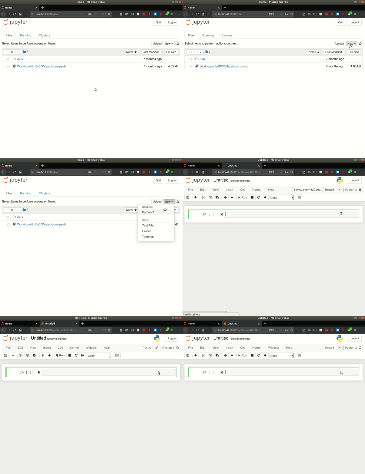
Now you can click New and select Python to create your first Jupyter notebook.
The code cells work similarly to IPython, except that these cells can be run
out of order, which is where confusion and errors may arise. But the real advantages
to notebooks are (1) in-line plotting with matplotlib and other plotting packages
and (2) you can convert code cells to Markdown cells that can be used to format
text to explain your code as you go along. This is where programming meets the
old-fashioned lab notebook (not coincidentally, the inspiration for the name).

Once again, code away young Padawan!
And check back for other posts and tutorials diving into the meat of programming in Python.